Bivariate Analysis

Bivariate analysis is the simultaneous analysis of two variables (attributes). Where univariate analysis asks “what does this variable look like?”, bivariate analysis asks “how do these two variables relate?” — whether an association exists, how strong it is, or whether two groups differ and whether that difference is significant.

This is the exploratory heart of explaining the past: most hypotheses about cause and effect in data begin life as a noticed association between two variables.

Three Combinations

There are three types of bivariate analysis, one for each pairing of variable types, and each has its own page in this section:

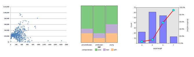
• Categorical vs. categorical — summarized with a contingency table, visualized with stacked column and combination charts, and tested for association with the chi-square test.
• Numerical vs. numerical — visualized with scatter plots (or a scatter plot matrix for many variables) and quantified with the linear (Pearson) correlation coefficient.
• Categorical vs. numerical — visualized with error-bar line charts, combination charts, and side-by-side box plots; group means are compared with the Z-test or t-test (two categories) and ANOVA (three or more).

Choosing the Right Tool

The pattern to internalize: the types of the two variables select the technique. A contingency table of two numerical variables is nonsense; a scatter plot of two categorical variables is a grid of dots. When a numerical variable must be analyzed against categories, analysts often bin it first (see Binning) — a legitimate move, but one that trades information for simplicity.

Also note the direction of inference: association is not causation. A strong chi-square result or a high correlation tells you the variables move together, not that one drives the other — confounding variables are the norm, not the exception.

In Practice

In pandas, pd.crosstab builds contingency tables, df.corr() the correlation matrix, and scipy.stats provides chi2_contingency, ttest_ind, and f_oneway for the significance tests; Seaborn’s heatmap, scatterplot, and boxplot cover the visuals. In machine-learning pipelines these same quantities power feature selection — sklearn.feature_selection.chi2 and mutual_info_classif rank predictors against a target using exactly the associations measured here.

Common Pitfalls

• Using the wrong technique for the type pair — correlation on categories, or chi-square on raw numbers.
• Confusing association with causation, especially when a lurking third variable explains both.
• Ignoring sample size. With enough rows, trivial associations become “statistically significant”; always look at effect size.
• Over-binning a numerical variable just to force it into a categorical analysis, destroying the very signal you were hunting.
• Multiple testing without care. Screen hundreds of variable pairs and some will look significant by chance alone.

Summary

Bivariate analysis examines two variables at once for association or group differences. The variable types choose the tool: contingency tables and chi-square for two categoricals, scatter plots and correlation for two numericals, error bars and mean-comparison tests for a categorical against a numerical. It is the bridge between describing data and modeling it.