Self-Organizing Maps

A Self-Organizing Map (SOM), or Kohonen network, projects high-dimensional data onto a low-dimensional grid — usually 1-D or 2-D — so it can be visualized and explored. It is unsupervised: there is no target vector, and the map learns to organize the data on its own. Its defining property is that it is topology preserving: points that are neighbors in the original space land near each other on the map.

Architecture

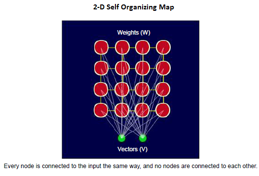
A SOM is a grid of nodes (units), each holding a weight vector with the same dimension as the input. Every node is connected to the input; the nodes are not connected to one another — their relationships live in the grid geometry itself.

A 2-D self-organizing map: a 4-by-4 grid of weight nodes, each connected to the input vectors; no connections between the nodes — A 2-D SOM: every grid node holds a weight vector and sees the whole input; nodes never connect to each other directly.

Training algorithm

Training iterates five steps, many thousands of times:

Initialize each node’s weight vector with small random values between 0 and 1.
Sample an input vector at random from the training set.
Find the Best Matching Unit (BMU) — the node whose weights are most similar to the input, measured by Euclidean distance:

$BMU = \arg\min_{v} \| D(t) - W_v(s) \|$

Compute the neighborhood radius around the BMU. The radius shrinks with time by an exponential decay, so early iterations move whole regions of the map while late ones fine-tune single nodes:

$\sigma(s) = \sigma_0 \, e^{-s / \lambda}$

Update the weights of the BMU and every node inside its neighborhood, pulling them toward the input. Nodes closer to the BMU move more, modulated by an influence function $\theta$ (1 inside the radius in the simplest form, commonly a Gaussian) and a decaying learning rate $\alpha(s) = \alpha_0 e^{-s/\lambda}$ :

$W_v(s+1) = W_v(s) + \theta(u, v, s)\, \alpha(s)\, \big( D(t) - W_v(s) \big)$

In the simplest form $\theta$ is 1 inside the radius and 0 outside; a Gaussian in the node’s grid distance from the BMU is the common refinement:

$\theta(t) = \exp\left( -\frac{dist^2}{2\sigma^2(t)} \right)$

As training proceeds, the neighborhood around the BMU shrinks exponentially until only the BMU itself is updated — global order first, local polish last.

From a random scatter of weights, iteration produces stable zones: regions of the grid specialized to regions of the input space. The final step — interpreting what each zone means — is done by a human; the SOM’s gift is making invisible structure visible.

SOM vs. k-means

Both partition data around prototype vectors, but k-means centroids are independent while SOM nodes sit on a grid and share updates with their neighbors. That coupling is what preserves topology — and what makes SOMs double as a clustering method and a dimensionality-reduction visualization. A SOM with a 1-D grid of $k$ nodes behaves much like k-means; a 2-D grid adds the map.

In practice

The classic implementation is MiniSom (pure Python, one file); for production-scale work, the update rule maps naturally to GPU frameworks. SOMs remain excellent for exploring high-dimensional omics, text embeddings, and sensor data — color the grid by node weight or hit count and structure jumps out. Modern alternatives for pure visualization (UMAP, t-SNE) compress better, but they give scatter plots, not a trainable grid of prototypes you can query, interpolate, and cluster with hierarchical methods.

Common pitfalls

Unnormalized inputs — the Euclidean BMU search is as scale-sensitive as k-NN’s.
Too few iterations: the map needs enough steps for the neighborhood to shrink through its full schedule, or it stays globally disordered.
A grid that’s too small, which crams distinct groups onto shared nodes; a grid that’s too large fragments real clusters.
Treating map distance as data distance — adjacent nodes are similar, but the grid is a projection, not the original space.
Reading clusters by eye without a hit histogram — count how many inputs map to each node before naming zones.

Summary

A self-organizing map trains a grid of weight vectors by repeatedly finding the Best Matching Unit for a sampled input and pulling the BMU and its exponentially shrinking neighborhood toward it. The result is a topology-preserving, low-dimensional view of high-dimensional data — part clustering algorithm, part visualization, and one of the most interpretable unsupervised tools going.