Support Vector Regression

Support Vector Regression (SVR) carries the maximal-margin idea of the support vector machine over to regression. The output is now a real number with infinitely many possible values, so the goal flips: instead of separating classes with the widest margin, fit a function that stays as flat as possible while keeping errors inside a tolerated band.

The epsilon-insensitive tube

Define a tube of half-width $\varepsilon$ around the fitted function. Errors inside the tube are ignored entirely — only points outside it count, through the ε-insensitive loss:

$L_\varepsilon(y, f(x)) = \max(0,\; |y - f(x)| - \varepsilon)$

For the linear case $f(x) = \langle w, x \rangle + b$, SVR minimizes the flatness term $\frac{1}{2}\|w\|^2$ plus a penalty $C$ on violations outside the tube, with slack variables $\xi_i, \xi_i^*$ absorbing the excess:

$\min_{w, b, \xi, \xi^*} \; \frac{1}{2}\|w\|^2 + C \sum_{i=1}^{N} (\xi_i + \xi_i^*)$

subject to

$y_i - \langle w, x_i \rangle - b \le \varepsilon + \xi_i, \qquad \langle w, x_i \rangle + b - y_i \le \varepsilon + \xi_i^*, \qquad \xi_i, \xi_i^* \ge 0$

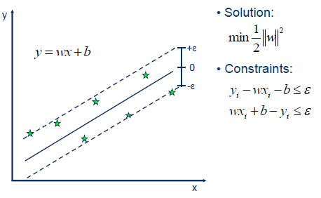
Two knobs shape the fit. ε sets the width of the indifference band — a larger ε tolerates more error and yields a flatter, smoother function. C trades flatness against tube violations — a larger C forces the function closer to the data. Only points on or outside the tube boundary contribute to the solution; these are the support vectors, which makes SVR robust to whatever happens deep inside the tube.

Non-linear SVR

When the relationship is curved, the kernel trick lifts the data into a higher-dimensional feature space where a linear tube fits — without ever computing the transformed coordinates. Because the optimization depends on the data only through inner products, any kernel function $K(x_i, x_j)$ can stand in for them. The common choices are the same as for classification:

$K(x_i, x_j) = (x_i \cdot x_j + 1)^d \quad \text{(polynomial)}, \qquad K(x_i, x_j) = e^{-\gamma \|x_i - x_j\|^2} \quad \text{(RBF)}$

The RBF kernel is the default: it fits local, non-linear structure with a single width parameter $\gamma$ to tune alongside $C$ and $\varepsilon$.

In practice

sklearn.svm.SVR (and the faster LinearSVR for large linear problems) implements ε-SVR with RBF, polynomial, and sigmoid kernels. Always scale features first — margin-based methods are scale-sensitive, so wrap the model in a Pipeline with StandardScaler. Tune the $(C, \varepsilon, \gamma)$ triple by grid search on cross-validated RMSE. SVR shines on small-to-medium datasets with smooth targets; on very large data it scales poorly (the kernel matrix is quadratic in $n$), where gradient-boosted trees or linear models on engineered features usually win.

Common pitfalls

• Unscaled features — the margin geometry is meaningless when one variable’s units dominate.
• Choosing ε without reference to the target’s scale: ε = 0.1 is generous for a target in [0, 1] and meaningless for one in thousands. Scale the target too, or set ε relative to its standard deviation.
• Huge C that chases every outlier, destroying the flatness that makes SVR robust.
• Expecting uncertainty bands — the ε-tube is a loss function, not a confidence interval; use quantile regression or Gaussian processes for calibrated intervals.
• Throwing SVR at millions of rows — kernel SVR training time grows roughly quadratically with $n$.

Summary

Support vector regression fits the flattest function whose ε-insensitive tube contains the data, penalizing only outside-tube violations via slack variables and the complexity budget $C$. Kernels extend the same tube to non-linear relationships. With proper scaling and a tuned $(C, \varepsilon, \gamma)$, SVR is a robust, outlier-tolerant regressor for moderate-size problems.