Univariate Analysis

Univariate analysis explores variables (attributes) one by one. It is the simplest form of data exploration and the mandatory first pass over any new dataset: before you ask how variables interact, you need to know what each one looks like on its own.

Variables are either categorical or numerical, and each type has its own statistical and visualization techniques. The goal in both cases is the same — describe the distribution of values compactly and honestly.

Two Types of Variables

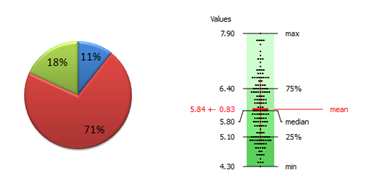
A categorical variable takes one of a fixed set of categories (for example, housing status: for free, own, rent). You summarize it with a frequency table — counts and percentages per category — and visualize it with a bar chart or pie chart.

A numerical variable takes values on a continuous or ordered numeric scale (for example, temperature or sepal length). You summarize it with measures of central tendency (mean, median, mode) and dispersion (variance, standard deviation, interquartile range), and visualize it with a histogram or box plot.

Crossing the Type Boundary

The two types are not walled off from each other, and two transformations appear constantly in data preparation:

• Binning (discretization) turns a numerical variable into a categorical one — for example, binning temperature into low / medium / high. See Binning.
• Encoding turns a categorical variable into numerical form — for example, one-hot encoding of categories into indicator columns. See Encoding.

Finally, proper handling of missing values is an important issue in mining data, and univariate analysis is where you first quantify them: a frequency table that omits the missing count is telling you a lie of omission.

In Practice

In Python, pandas.Series.describe() gives the full numerical summary, while value_counts() (with dropna=False) is the frequency table for categorical data; Seaborn’s histplot, boxplot, and countplot cover the visuals. Tree-based libraries like XGBoost consume raw numerical and encoded categorical features directly, but your choice of encoding or binning strategy still shapes linear models and neural networks — and it starts with what you learn here.

Common Pitfalls

• Applying numerical statistics to categories. The “mean” of an encoded categorical variable (e.g., average zip code) is meaningless.
• Ignoring missing values in counts and percentages, which silently inflates the observed categories.
• Reading shape from summary statistics alone. Mean and SD cannot tell a bimodal distribution from a normal one — always plot.
• Treating IDs as variables. Unique identifiers have one value per row; they carry no distribution to explore.
• Forgetting units and scale when comparing summaries across variables.

Summary

Univariate analysis profiles one variable at a time: frequency tables and bar charts for categorical variables, summary statistics with histograms and box plots for numerical ones. Binning and encoding convert between the two types, and missing-value counts belong in every summary. Master this pass and every later analysis — bivariate, modeling, evaluation — gets easier.