Model Deployment

Deployment in data science means applying a trained model to new data. Building the model is generally not the end of the project — even when its purpose was simply to understand the data, the knowledge gained must be organized and presented so the customer can use it. Depending on requirements, deployment can be as simple as generating a report or as complex as implementing a repeatable, production data science process.

Often it is the customer, not the analyst, who carries out the deployment steps — a credit card company, for instance, may deploy a trained neural network to flag transactions with a high probability of fraud in real time. That is why deployment must be planned from the start: the customer needs to understand up front what actions are required to actually make use of the models.

The four deployment methods

There are, in general, four ways to deploy a model:

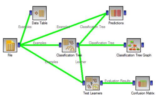
1. A data science tool (or cloud service) — the model stays inside the platform where it was built and scores data there. Below, a decision tree deployed in the Orange data mining tool.
2. A programming language — the model’s logic is reimplemented or exported as code (Java, C, Python) and embedded directly in an application.
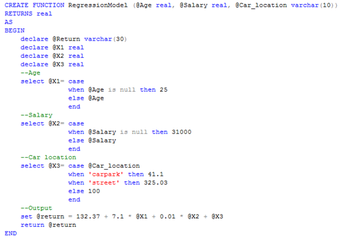
3. Database and SQL script — the model is expressed as SQL (TSQL, PL/SQL) so scoring happens where the data lives.
4. PMML — the model is exported to a standard interchange format and consumed by any compliant scoring engine.

PMML: the portable model format

PMML (Predictive Model Markup Language) is an XML-based language for defining statistical and data mining models and sharing them between compliant applications. Developed by the DMG (Data Mining Group), it defines a standard not only for representing models but also for data handling and pre/post-processing. PMML eliminates custom, one-off deployment work and cleanly separates model development from model deployment. Supported techniques include regression, neural networks, support vector machines, decision trees, naive Bayes, clustering, sequences, rule sets, association rules, time series, and text models.

Where the legacy page showed PMML as screenshots, here is the substance as actual markup — the skeleton of a deployed regression model:

<PMML version="4.4">
  <Header copyright="Bioada" description="Regression model"/>
  <DataDictionary numberOfFields="2">
    <DataField name="age" optype="continuous" dataType="double"/>
    <DataField name="risk" optype="continuous" dataType="double"/>
  </DataDictionary>
  <RegressionModel modelName="riskScore" functionName="regression">
    <MiningSchema>
      <MiningField name="age" usageType="active"/>
      <MiningField name="risk" usageType="predicted"/>
    </MiningSchema>
    <RegressionTable intercept="0.42">
      <NumericPredictor name="age" coefficient="0.013"/>
    </RegressionTable>
  </RegressionModel>
</PMML>

PMML components

• Header — general document information: copyright, model description, the generating application’s name and version, and a creation timestamp.
• Data dictionary — definitions of every field the model may use: whether each is continuous, categorical, or ordinal, plus valid value ranges and data types.
• Data transformations — mappings from raw user data into model-ready form: normalization, discretization, value mapping, derived functions, and aggregation.
• Model — the model itself; a neural network, for example, is a NeuralNetwork element carrying its name, function, algorithm, activation function, and number of layers.
• Mining schema — the subset of dictionary fields the model actually uses, each with a usage type (active, predicted, supplementary), outlier treatment, and missing-value policy.
• Targets — post-processing of the predicted value: scaling continuous outputs, or specifying prior probabilities for classification when the prediction logic produces no result (e.g., a missing input).

Later PMML versions added richer pre-processing, time series models, embedded evaluation metrics, ensembles and model composition, and multi-class SVMs — but the component structure above is the enduring core.

In practice

The four legacy paths survive, modernized: models are exported with sklearn2pmml or ONNX (sklearn-onnx), served as REST endpoints from a Docker container, or scored in-database with SQL or tools like BigQuery ML and Snowflake. The discipline around deployment is now called MLOps: version the model alongside its training data and code, monitor input distributions for drift and predictions for degradation, and keep a rollback path. A model that cannot be monitored and retrained is not deployed — it is abandoned.

Common pitfalls

• Training/serving skew — features computed one way in training and another in production.
• Reimplementing model logic by hand in application code instead of exporting a portable artifact (PMML, ONNX).
• Deploying without monitoring: silent data drift erodes accuracy for months before anyone notices.
• No versioning or rollback, so a bad retrain cannot be undone.
• Leaving the customer out of deployment planning — the people who operate the model must be ready before go-live.

Summary

Deployment applies a validated model to new data, and it belongs in the plan from day one. The four classic paths — tools, code, SQL, and PMML — have modern equivalents in ONNX, containers, and in-database scoring, and the job ends not at go-live but with monitoring, drift detection, and retraining. For how models earn the right to be deployed, see model evaluation.