Numerical Variables

A numerical (or continuous) variable is one that may take on any value within a finite or infinite interval — height, weight, temperature, blood glucose, and so on. Where categorical variables are summarized by counting, numerical variables are summarized by measuring: where is the center, how wide is the spread, and what shape does the distribution take?

Interval and Ratio Variables

There are two types of numerical variable. An interval variable has values whose differences are interpretable, but it has no true zero — temperature in degrees Centigrade is the classic case. Interval data can be added and subtracted but not meaningfully multiplied or divided: you cannot say that one day is twice as hot as another. A ratio variable has a true zero and supports all four arithmetic operations — weight is a good example, and 20 kg really is twice 10 kg.

Central Tendency

The mean is the sum of the values divided by the count:

$\bar{x} = \frac{1}{n} \sum_{i=1}^{n} x_i$

The median is the middle value of the sorted data — below and above it lies an equal number of values. For sorted values $x_{(1)} \le \dots \le x_{(n)}$:

$\tilde{x} = \begin{cases} x_{\left(\frac{n+1}{2}\right)} & n \text{ odd} \\ \frac{1}{2}\left(x_{\left(\frac{n}{2}\right)} + x_{\left(\frac{n}{2}+1\right)}\right) & n \text{ even} \end{cases}$

The mode is the most frequent value; there can be more than one. The median is robust to outliers while the mean is not — when they disagree, the distribution is skewed or contaminated, and the gap is itself a finding.

Dispersion

The range is $\max - \min$. The variance measures average squared distance from the mean:

$s^2 = \frac{\sum_{i=1}^{n} (x_i - \bar{x})^2}{n - 1}$

and the standard deviation is its square root, $s = \sqrt{s^2}$, which returns the measure to the original units. The coefficient of variation expresses dispersion relative to the mean, making spread comparable across variables of different scales:

$cv = \frac{s}{\bar{x}}$

Quantiles are cut points dividing the sorted data into groups of equal size — quartiles (4 groups), quintiles (5), percentiles (100). The interquartile range, $\mathrm{IQR} = Q_3 - Q_1$, spans the middle 50% of the data and is the dispersion measure behind the box plot.

Shape

Skewness measures asymmetry of the distribution — positive skew means a long right tail, negative skew a long left tail:

$g_1 = \frac{n}{(n-1)(n-2)} \sum_{i=1}^{n} \left( \frac{x_i - \bar{x}}{s} \right)^3$

Kurtosis measures whether the data are peaked or flat relative to a normal distribution (a normal distribution has excess kurtosis of 0):

$g_2 = \frac{n(n+1)}{(n-1)(n-2)(n-3)} \sum_{i=1}^{n} \left( \frac{x_i - \bar{x}}{s} \right)^4 - \frac{3(n-1)^2}{(n-2)(n-3)}$

Visualization

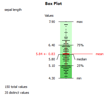
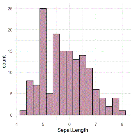
The histogram bins the values and plots a bar per bin — it reveals modality, skew, and outliers at a glance. The box plot compresses the distribution into five numbers: the box spans $Q_1$ to $Q_3$ with a line at the median, whiskers extend toward the extremes (typically $1.5 \times \mathrm{IQR}$), and points beyond are drawn individually as outlier candidates.

Worked Example: Iris Sepal Length

The legacy example analyzes the sepal length variable from the Iris dataset ($n = 150$):

Statistic	Value
Count	150
Minimum	4.3
Maximum	7.9
Mean	5.84
Median	5.8
Mode	5.0
Quartile 1	5.1
Range	3.6
Variance	0.69
Standard Deviation	0.83
Coefficient of Variation	14.2%
Skewness	0.31
Kurtosis	−0.55

Read together: the mean (5.84) sits just above the median (5.8), consistent with the mild positive skewness (0.31); the CV of 14.2% says the spread is modest relative to the center; and the negative excess kurtosis (−0.55) indicates slightly flatter tails than a normal curve.

In Practice

df.describe() in pandas returns count, mean, std, min, quartiles, and max in one call; scipy.stats.skew and scipy.stats.kurtosis add shape. These summaries feed directly into modeling decisions: heavy skew motivates log transforms before linear regression, outliers visible in a box plot motivate robust scalers, and standardization (subtracting $\bar{x}$, dividing by $s$) is the default preprocessing for SVMs, k-NN, and neural networks.

Common Pitfalls

• Reporting the mean of a skewed variable without the median — one outlier can pull the mean far from the typical value.
• Comparing standard deviations across variables with different scales; use the coefficient of variation instead.
• Trusting statistics without the plot. Anscombe-style pathologies hide from summary numbers; always look at the histogram.
• Mixing up population and sample variance ($n$ vs. $n-1$ in the denominator) when comparing tools — Excel’s VAR.P/VAR.S differ for exactly this reason.
• Reading kurtosis as “peakedness” alone — it is dominated by tail weight, and only meaningful on a decent sample size.

Summary

Numerical variables are interval or ratio, and their univariate profile has three layers: central tendency (mean, median, mode), dispersion (range, variance, standard deviation, IQR), and shape (skewness, kurtosis). The histogram and box plot make all three visible, and the Iris example shows how the numbers and pictures corroborate each other.