Support Vector Machine

A Support Vector Machine (SVM) classifies by finding the hyperplane that separates two classes with the widest possible margin — the broadest empty band between the classes. Where logistic regression fits all the data to maximize likelihood, an SVM cares only about the handful of cases closest to the boundary, which makes it robust and data-efficient.

The cases that touch the margin’s edges are the support vectors. They alone define the hyperplane: remove any other training point and the model doesn’t move; move a support vector and it does.

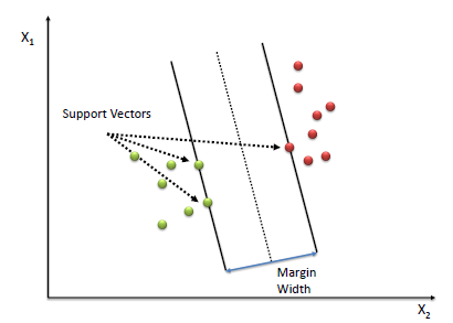
Maximum-margin optimization

Write the hyperplane as $w \cdot x + b = 0$, with class labels $y_i \in \{-1, +1\}$. The margin width is $\frac{2}{\lVert w \rVert}$, so maximizing the margin means minimizing $\lVert w \rVert$ while keeping every case correctly classified outside the band:

$\min_{w,\, b} \; \frac{1}{2} \lVert w \rVert^2 \quad \text{subject to} \quad y_i\,(w \cdot x_i + b) \geq 1 \;\; \text{for all } i$

This is a quadratic programming problem with a unique global minimum when the data is linearly separable — no local-optima lottery, unlike neural network training.

Real data rarely separates perfectly, so the soft-margin formulation adds slack variables $\xi_i$ that price each violation, trading margin width against misclassification:

$\min_{w,\, b,\, \xi} \; \frac{1}{2} \lVert w \rVert^2 + C \sum_{i=1}^{n} \xi_i \quad \text{subject to} \quad y_i\,(w \cdot x_i + b) \geq 1 - \xi_i, \;\; \xi_i \geq 0$

The parameter $C$ is the trade-off knob: large $C$ punishes violations hard (narrow margin, low bias, risk of overfitting); small $C$ tolerates violations for a wider, smoother margin. Equivalently, training minimizes hinge loss plus a ridge penalty:

$\ell(y, f(x)) = \max\big(0,\; 1 - y\, f(x)\big)$

Hinge loss is zero once a case is classified correctly with confidence — which is exactly why only the boundary-adjacent cases end up mattering.

The kernel trick

Some boundaries no straight hyperplane can draw. The SVM answer: map the data into a higher-dimensional feature space where a linear separator does exist, then let the classifier work there.

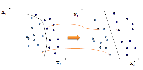
The elegant part is that the optimization only ever needs inner products between cases — never the transformed coordinates themselves. A kernel function computes those inner products in the high-dimensional space directly, without ever visiting it: $\langle \phi(x), \phi(y) \rangle = K(x, y)$. So a nonlinear function is learned by a linear machine, at the cost of computing only dot products in the original space. Two standard kernels:

• Polynomial: $K(x, y) = (x \cdot y + c)^d$
• Radial basis function (RBF / Gaussian):

$K(x, y) = \exp\!\big(-\gamma \lVert x - y \rVert^2\big)$

The RBF kernel’s $\gamma$ controls reach: large $\gamma$ gives each support vector a tight, local influence (wiggly boundary); small $\gamma$ smooths globally. Together, $C$ and $\gamma$ are the two hyperparameters every SVM practitioner tunes.

In practice

sklearn.svm.SVC is the general-purpose implementation (kernel='rbf' by default); LinearSVC scales much better for large linear problems, and SGDClassifier(loss='hinge') approximates an SVM on data too big for either. Always standardize features first — margins are distances, and unscaled features corrupt them exactly as in k-NN. Tune $C$ and $\gamma$ on a log-scale grid with cross-validation. SVMs output scores, not probabilities; wrap in CalibratedClassifierCV when you need calibrated risk estimates. Kernel SVMs remain competitive on small-to-medium tabular datasets, though boosted trees usually win at scale.

Common pitfalls

• Skipping feature scaling. A margin is a geometric object; mixed units distort it beyond recognition.
• Cranking $C$ up to fit the training set. Large $C$ on noisy data overfits exactly the cases that should be tolerated as violations.
• Default $\gamma$ on tiny or huge datasets. gamma='scale' is a reasonable start, but it must be tuned jointly with $C$.
• Expecting probabilities. Raw SVM outputs are signed distances; calibrate before thresholding for risk.
• Quadratic training cost. Kernel SVMs scale poorly past ~100k cases — switch to linear or SGD variants.

Summary

An SVM finds the hyperplane with the maximum margin, defined entirely by the support vectors on its boundary. Soft margins with slack variables (equivalently, hinge loss) handle inseparable data, with $C$ mediating the fit-versus-simplicity trade-off. The kernel trick — above all the RBF kernel $K(x,y) = e^{-\gamma \lVert x-y \rVert^2}$ — lifts the same linear machinery into nonlinear territory at dot-product cost.