Hierarchical Clustering

Hierarchical clustering produces clusters with a built-in ordering from top to bottom — the way files and folders nest on a disk. Instead of one flat partition, you get a whole spectrum of them, summarized in a dendrogram that you cut at whatever height gives a useful number of clusters. There are two directions for building the tree:

• Divisive (top-down): assign every observation to one cluster, split it into the two least similar parts with a flat method such as k-means, and recurse until each observation stands alone. Divisive methods can produce more accurate hierarchies but are conceptually and computationally heavier.
• Agglomerative (bottom-up): start with each observation in its own cluster, merge the two most similar clusters, and repeat until one cluster remains. This is the common form, and the one we work through below.

Linkage: defining distance between clusters

Agglomerative merging needs a distance between clusters, not just points. The three classic linkage rules:

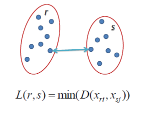
• Single linkage — the shortest distance between any two points in the two clusters. Prone to chaining: clusters merge through bridges of nearby points.
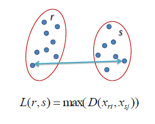
• Complete linkage — the longest distance between any two points. Produces compact, tight clusters but is sensitive to outliers.
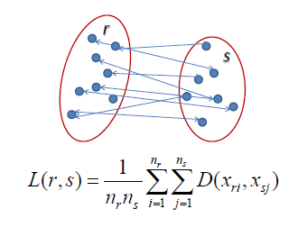
• Average linkage — the average distance over all cross-cluster point pairs. A robust middle ground, and the most common default.

Worked example: seven points

Cluster these seven 2-D points with Euclidean distance and average linkage:

Point	$X_1$	$X_2$
A	10	5
B	1	4
C	5	8
D	9	2
E	12	10
F	15	8
G	7	7

Step 1 — proximity matrix. Compute every pairwise distance (lower triangle shown):

	A	B	C	D	E	F
B	9.06
C	5.83	5.66
D	3.16	8.25	7.21
E	5.39	12.53	7.28	8.54
F	5.83	14.56	10.00	8.49	3.61
G	3.61	6.71	2.24	5.39	5.83	8.06

The shortest distance is $d(C, G) = 2.24$ — merge {C, G}.

Step 2 — update and repeat. With average linkage, the distance from a merged cluster to a point is the mean of the pairwise distances — e.g. $d(\{C,G\}, A) = (5.83 + 3.61)/2 = 4.72$. The next minimum is $d(A, D) = 3.16$ — merge {A, D}. Then $d(E, F) = 3.61$ — merge {E, F}.

Step 3 — keep going. The distance between {A, D} and {C, G} averages the four cross pairs: $(5.83 + 3.61 + 7.21 + 5.39)/4 = 5.51$ — the smallest entry, so merge {A, D, C, G}.

Step 4 — nearly tied. Now $d(B, \{A,D,C,G\}) = 7.42$ and $d(\{E,F\}, \{A,D,C,G\}) = 7.43$ — B wins by a hair and merges at 7.42, leaving {E, F} to join last at 8.65, which completes the tree.

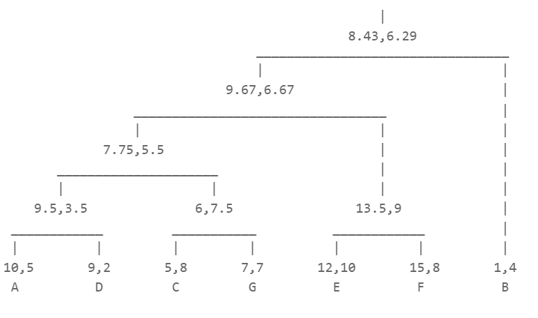
To read a dendrogram, draw a horizontal line: every vertical branch it crosses is a cluster. Cutting high gives few coarse clusters; cutting low gives many fine ones.

In practice

sklearn.cluster.AgglomerativeClustering supports single, complete, average, and Ward linkage (scipy.cluster.hierarchy.linkage + dendrogram gives the classic plot and cut tools). Ward’s method — merging the pair that least increases within-cluster variance — is the practical default for Euclidean data. The $O(n^2)$ proximity matrix caps plain agglomerative clustering at tens of thousands of points; sample or use BIRCH beyond that. Choose the cut with the dendrogram plus a silhouette sweep rather than by eye alone.

Common pitfalls

• Forgetting to scale — the proximity matrix inherits the units of your features.
• Assuming the dendrogram is unique — linkage choice, ties, and even point ordering can reshape the top of the tree (see the 7.42/7.43 near-tie above).
• Chaining with single linkage on noisy data, producing one long snake instead of groups.
• Cutting by eye only; confirm the chosen level with an internal metric.
• Feeding it millions of points — hierarchical clustering is $O(n^2)$ space and roughly $O(n^3)$ naive time.

Summary

Hierarchical clustering nests clusters into a dendrogram: divisive methods split top-down, agglomerative methods merge bottom-up using a linkage rule — single, complete, or average — to measure distance between clusters. On seven points with average linkage, {C, G}, {A, D}, and {E, F} form first, then combine; cut the tree where the structure is stable, and always remember the tree depends on the linkage you chose.