Decision Tree Regression

A regression tree uses the same top-down, greedy induction as a classification tree — break the dataset into smaller and purer subsets while growing a tree of decision nodes and leaf nodes — but predicts a number: each leaf holds the average target of the cases that reach it. The only algorithmic change is the splitting criterion.

Standard deviation reduction

For classification, ID3 chooses splits by information gain. A numerical target has no class counts to compute entropy from, so Quinlan’s algorithm swaps in standard deviation reduction (SDR): split on the attribute whose branches are most homogeneous in the target.

Standard deviation measures the homogeneity of a numerical sample — a perfectly homogeneous subset has $S = 0$:

$S = \sqrt{\frac{\sum_{i=1}^{n}(x_i - \bar{x})^2}{n}}$

Three derived statistics drive the algorithm:

• S — the standard deviation, used to score candidate splits.
• CV — the coefficient of variation, $CV = \frac{S}{\bar{x}} \times 100\%$, used as a stopping rule (branching stops when a node is homogeneous enough).
• Avg — the mean, the value assigned to a leaf.

The expected standard deviation after splitting set $T$ on attribute $X$ is the weighted average of the branch deviations, and SDR is the drop:

$S(T, X) = \sum_{c \in X} P(c)\, S(c), \qquad SDR(T, X) = S(T) - S(T, X)$

Worked example: predicting hours played

The classic golf dataset, with Hours Played as the numerical target (note the legacy Sunny/Rainy labeling):

Outlook	Temp	Humidity	Windy	Hours Played
Rainy	Hot	High	False	25
Rainy	Hot	High	True	30
Overcast	Hot	High	False	46
Sunny	Mild	High	False	45
Sunny	Cool	Normal	False	52
Sunny	Cool	Normal	True	23
Overcast	Cool	Normal	True	43
Rainy	Mild	High	False	35
Rainy	Cool	Normal	False	38
Sunny	Mild	Normal	False	46
Rainy	Mild	Normal	True	48
Overcast	Mild	High	True	52
Overcast	Hot	Normal	False	44
Sunny	Mild	High	True	30

Step 1 — root deviation. The standard deviation of all 14 values is $S(\text{Hours}) = 9.32$.

Step 2 — score each attribute. Splitting on Outlook gives branch deviations 3.49 (Overcast), 7.78 (Rainy), 10.87 (Sunny), so $S(\text{Hours}, \text{Outlook}) = \frac{4(3.49) + 5(7.78) + 5(10.87)}{14} = 7.66$:

$SDR(\text{Hours}, \text{Outlook}) = 9.32 - 7.66 = 1.66$

The other candidates are weaker — Temp 0.48, Humidity 0.27, Windy 0.28 — so Outlook becomes the root node.

Step 3 — recurse with stopping rules. In practice we stop splitting a branch when its CV falls below a threshold (say 10%) or too few instances remain (say 3).

• Overcast $\{46, 43, 52, 44\}$: CV = 8% < 10% — stop. Leaf = average 46.3.
• Sunny $\{45, 52, 23, 46, 30\}$: CV = 28% — split again. Windy has the largest SDR here (7.62): Windy=False $\{45, 52, 46\}$ → 47.7; Windy=True $\{23, 30\}$ → 26.5. Both branches now have ≤ 3 instances, so stop.
• Rainy $\{25, 30, 35, 38, 48\}$: CV = 22% — split again. Temp has the largest SDR (4.18): Cool → 38, Hot $\{25, 30\}$ → 27.5, Mild $\{35, 48\}$ → 41.5.

The finished tree, with the dataset it was built from:

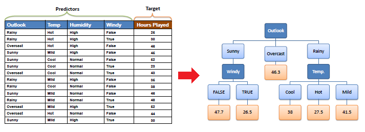
When a leaf contains more than one instance, its prediction is simply the branch average — the least-squares optimal constant for that subset.

In practice

sklearn.tree.DecisionTreeRegressor implements the same idea with variance reduction (equivalent to SDR) or absolute-error criteria, plus pruning controls like min_samples_leaf and max_depth that play the role of the CV threshold. Single regression trees overfit easily, which is why they are mostly used as base learners: random forests and gradient-boosted trees (XGBoost, LightGBM) average or stage hundreds of them and dominate tabular regression benchmarks. Inspect any tree model with SHAP values to see how each feature moves the prediction.

Common pitfalls

• No stopping rule — an unpruned tree grows one leaf per instance and memorizes the training set.
• Thresholds that are too strict — a high CV cutoff or large minimum count underfits, collapsing real structure into a stump.
• Instability: a small change in the data can flip the root split and restructure the whole tree. Never read deep causal meaning into one tree.
• Piecewise-constant predictions — a tree cannot extrapolate a trend beyond the range it has seen; use linear models or boosted stumps when smoothness matters.
• Ignoring leaf counts — a leaf averaging 2 cases is a guess, not a pattern.

Summary

Regression trees reuse the ID3 greedy search with standard deviation reduction in place of information gain: split where branches become most homogeneous, stop on CV or instance count, and predict the leaf average. On the golf data, Outlook (SDR 1.66) anchors a small tree that predicts hours played within about ±10 of the true value — and the same machinery scales up to the ensemble methods that power modern tabular regression.