Categorical Variables

A categorical (or discrete) variable is one that has two or more categories (values). Because the values are labels rather than quantities, the whole game of univariate analysis here is counting: how often does each category occur, and what share of the data does it represent?

Nominal and Ordinal Variables

There are two types of categorical variable:

• A nominal variable has no intrinsic ordering to its categories. For example, gender is a categorical variable with two categories (male and female) and no meaningful order between them.
• An ordinal variable has a clear ordering. For example, temperature binned into three orderly categories (low, medium, high) is ordinal: medium sits between low and high, but the “distance” between categories is undefined.

Statistics and Visualization

Statistic	Visualization	Description
Count	Bar chart	The number of values of the specified variable.
Count %	Pie chart	The percentage of values of the specified variable.

The bar chart is the workhorse: one bar per category, height proportional to count or percentage, and — unlike a histogram — gaps between bars to emphasize that categories are discrete. A pie chart shows the same percentages as slices; it is readable for a handful of categories but degrades quickly as categories multiply, and comparing slice angles is harder for the eye than comparing bar heights.

Worked Example: Housing

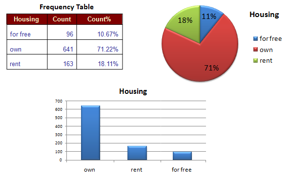
The legacy example uses a housing variable with three categories: for free, own, and rent. The frequency table:

Housing	Count	Percentage
for free	96	10.67%
own	641	71.22%
rent	163	18.11%
Total	900	100.00%

The percentages are just each count divided by the total: for example, $\frac{96}{900} \times 100 = 10.67\%$. The story is immediate — nearly three quarters of respondents own their housing — and it is exactly the kind of first-glance fact that shapes every later modeling decision about this feature.

In Practice

pandas.Series.value_counts() (with normalize=True for percentages) produces the frequency table in one line, and sns.countplot the bar chart. Before feeding categories to a model you will typically encode them — see Encoding — or, in the other direction, create categorical variables from numerical ones via Binning. Tree libraries such as LightGBM and CatBoost can consume categorical features natively, which makes knowing your category inventory upfront even more valuable.

Common Pitfalls

• Computing numeric summaries of categories. There is no mean or standard deviation of a nominal variable — only counts, percentages, and the mode.
• Hiding rare levels. Long tails of tiny categories distort percentages and charts; consider an “other” bucket.
• Treating ordinal as nominal. Order is information — preserve it when encoding.
• Overusing pie charts. More than about five slices, and a bar chart communicates better.
• Forgetting the missing category. Missing values deserve their own row in the frequency table.

Summary

Categorical variables come in nominal and ordinal flavors, and univariate analysis of them reduces to counting: a frequency table with counts and percentages, drawn as a bar or pie chart. The housing example shows how much a single table can tell you — distribution, dominance, and rare levels — before any modeling begins.