Evaluation: Regression

After building several regression models, you need criteria to evaluate and compare them. Regression metrics fall into two families: absolute error measures in the units of the target (MAE, MSE, RMSE), which compare models predicting the same quantity, and relative measures (RSE, RAE, $R^2$), which are unit-free and compare across datasets. Throughout, $a_i$ is the actual target and $p_i$ the predicted target for observation $i$ of $n$. As with classification, these scores are only meaningful on held-out data — see Model Evaluation.

Absolute error metrics

The mean absolute error averages the unsigned errors. It has the same unit as the original data and is easy to interpret:

$$\text{MAE} = \frac{\sum_{i=1}^{n} |p_i - a_i|}{n}$$

The mean squared error squares the errors before averaging, penalizing large misses much more than small ones:

$$\text{MSE} = \frac{\sum_{i=1}^{n} (p_i - a_i)^2}{n}$$

The root mean squared error takes the square root of MSE to return to the original units:

$$\text{RMSE} = \sqrt{\frac{\sum_{i=1}^{n} (p_i - a_i)^2}{n}}$$

RMSE is the most popular error measure for regression, but it can only be compared between models whose errors are measured in the same units. MAE is usually similar in magnitude to RMSE but slightly smaller — the squaring inflates RMSE whenever errors vary in size.

Relative metrics and R²

The relative squared error and relative absolute error normalize by the error of a naive baseline that always predicts the mean $\overline{a}$, so they can be compared across models whose targets have different units:

$$\text{RSE} = \frac{\sum_{i=1}^{n} (p_i - a_i)^2}{\sum_{i=1}^{n} (\overline{a} - a_i)^2} \qquad \text{RAE} = \frac{\sum_{i=1}^{n} |p_i - a_i|}{\sum_{i=1}^{n} |\overline{a} - a_i|}$$

The coefficient of determination, $R^2$, is the most widely reported relative measure. Writing $\text{SSE} = \sum_{i=1}^{n}(p_i - a_i)^2$ and $\text{SST} = \sum_{i=1}^{n}(\overline{a} - a_i)^2$:

$$R^2 = 1 - \frac{\text{SSE}}{\text{SST}}$$

$R^2$ is the proportion of the dependent variable’s variance explained by the model. If the model is perfect, SSE is zero and $R^2 = 1$; if the model is a total failure — no better than predicting the mean — SSE equals SST and $R^2 = 0$.

Worked example

A model predicts five observations; actual and predicted targets are:

| $i$ | $a_i$ (actual) | $p_i$ (predicted) | $p_i - a_i$ | $|p_i - a_i|$ | $(p_i - a_i)^2$ | | --- | --- | --- | --- | --- | --- | | 1 | 3 | 2 | $-1$ | 1 | 1 | | 2 | 5 | 6 | $1$ | 1 | 1 | | 3 | 2 | 3 | $1$ | 1 | 1 | | 4 | 8 | 7 | $-1$ | 1 | 1 | | 5 | 7 | 7 | $0$ | 0 | 0 | | Sum | 25 | | | 4 | 4 |

The mean of the actual values is $\overline{a} = 25/5 = 5$, so the baseline terms are $\sum(\overline{a} - a_i)^2 = 4 + 0 + 9 + 9 + 4 = 26$ and $\sum|\overline{a} - a_i| = 10$. Then:

$$\text{MAE} = \frac{4}{5} = 0.80 \qquad \text{MSE} = \frac{4}{5} = 0.80 \qquad \text{RMSE} = \sqrt{0.80} \approx 0.89$$ $$\text{RSE} = \frac{4}{26} \approx 0.15 \qquad \text{RAE} = \frac{4}{10} = 0.40 \qquad R^2 = 1 - \frac{4}{26} \approx 0.85$$

Note RMSE ($\approx 0.89$) sitting slightly above MAE ($0.80$), exactly as expected, and $R^2 \approx 0.85$ saying the model explains about 85% of the variance that the mean-only baseline leaves unexplained.

Residual plots

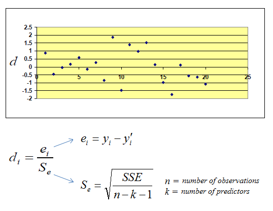
Numbers compress; plots reveal. A residual plot charts the residuals $e_i = a_i - p_i$ (or their standardized versions) against fitted values or observation order. A healthy model shows a shapeless band around zero; curves, funnels, or clusters in the band mean the model is missing structure. The standardized residual divides by the residual standard error,

$$d_i = \frac{e_i}{S_e} \qquad S_e = \sqrt{\frac{\text{SSE}}{n - k - 1}}$$

where $k$ is the number of predictors. Standardization puts residuals on a common scale so potential outliers — typically $|d_i| > 2$ or $3$ — stand out immediately.

In practice

In scikit-learn, sklearn.metrics.mean_absolute_error, mean_squared_error, root_mean_squared_error, and r2_score compute every metric on this page, and cross_val_score with scoring="neg_root_mean_squared_error" evaluates them under cross-validation. Which metric to optimize is a modeling decision: RMSE matches models trained by least squares (like the regression-fitting objective), while MAE is robust to outliers and matches median regression; XGBoost and LightGBM let you pick either as the training objective. Always inspect residual plots — statsmodels and yellowbrick have ready-made diagnostics — because two models with identical RMSE can fail in very different ways.

Common pitfalls

• Comparing RMSE across datasets or targets. Error in dollars and error in kilograms are incomparable; use RSE, RAE, or $R^2$ for cross-dataset comparison.
• Chasing $R^2$ alone. A high $R^2$ on training data can hide overfitting; report it on held-out folds.
• Ignoring units and scale. An RMSE of 0.89 is meaningless without knowing whether the target ranges over 0–10 or 0–10,000.
• Letting outliers dominate. Squared-error metrics can be dictated by a handful of extreme errors; check residuals and consider MAE.
• Adding predictors to inflate $R^2$. On training data $R^2$ never decreases when you add features; adjusted $R^2$ or a test-set score corrects this.

Summary

MAE, MSE, and RMSE measure average error in the target’s own units; RSE, RAE, and $R^2$ normalize against a mean-only baseline so models can be compared across datasets. The worked example shows all six computed from the same five predictions. Pair every numeric score with a residual plot — the numbers tell you how much a model errs, the plot tells you how.