Neural Networks

An artificial neural network (ANN) is a learning system loosely modeled on the brain. A biological neuron receives signals through thousands of synapses, sums them, and fires when the total crosses a threshold; an artificial neuron does the same with numbers. The brain’s roughly 100 billion neurons dwarf any artificial network, but the computational mirror — weighted sums, thresholds, and error-driven adjustment — turns out to be remarkably powerful.

The artificial neuron

A network is made of nodes organized in three roles: input nodes that receive the predictors as numbers, hidden nodes that transform them, and output nodes that produce the prediction. Connections carry weights — positive (excitatory) or negative (inhibitory) — that encode what the network has learned.

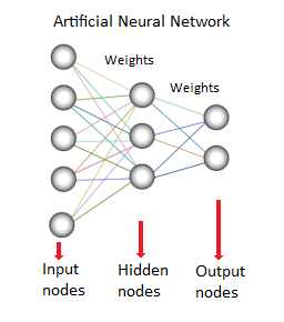
Each node computes a weighted sum of its inputs plus a bias, then applies a transfer (activation) function $f$:

$y = f\!\left(\sum_{i=1}^{n} w_i x_i + b\right)$

The simplest such unit, the perceptron, uses a unit step for $f$: output 1 if the weighted sum exceeds the threshold, 0 otherwise. A perceptron alone can only learn linearly separable boundaries; stacking neurons into hidden layers is what unlocks nonlinear decision surfaces.

Activation functions

The transfer function shapes each neuron’s response. Four families are common:

• Unit step (threshold). Two levels, on or off. Historically important (the original perceptron), but its zero gradient makes it untrainable by gradient methods.

• Sigmoid (logistic). Smooth and bounded in $(0, 1)$ — the same curve as logistic regression:

  $\sigma(z) = \frac{1}{1 + e^{-z}}$

  Its hyperbolic-tangent sibling, $\tanh(z)$, spans $(-1, 1)$ and centers its output at zero.

• Piecewise linear. Output proportional to input within a bounded range.

• Gaussian. A bell curve peaked at a chosen center — the basis of radial basis function networks.

Modern deep networks overwhelmingly prefer the rectified linear unit (ReLU):

$f(z) = \max(0, z)$

ReLU is cheap to compute, doesn’t saturate for positive inputs, and its constant gradient keeps deep stacks trainable.

Learning: backpropagation in brief

Training is gradient descent on the prediction error. For each example, the network produces an output; the gap between prediction and truth defines a loss. That error is then propagated backward through the network: using the chain rule, each weight receives a share of blame proportional to how much it contributed to the error, and every weight is nudged downhill against its gradient. Repeated over many examples and many passes, the weights converge to values that map inputs to correct outputs.

Two broad architectures matter:

• Feed-forward networks (perceptrons, multilayer perceptrons, radial basis function networks) pass signals in one direction only — input to hidden to output. These are the workhorses of data mining.
• Feed-back (recurrent) networks contain loops, so signals can circulate; they behave as nonlinear dynamic systems settling toward equilibrium, and historically powered associative memories and sequence models.

From perceptrons to transformers

The multilayer perceptron you just met is the direct ancestor of every modern deep network. The deep-learning revolution of the 2010s was, at heart, the same neurons and the same backpropagation — scaled up with ReLU activations, better initializations, GPUs, and vastly more data. Convolutional networks added weight-sharing for images, recurrent networks added memory for sequences, and in 2017 the transformer replaced recurrence with attention: a mechanism that lets every position in a sequence weigh every other position directly, capturing long-range structure that MLPs and RNNs struggle with. Transformers now dominate language, vision, and increasingly tabular and biological sequence modeling. Yet the fundamentals on this page — weighted sums, nonlinear activations, loss gradients flowing backward — are unchanged; every transformer is still trained by backpropagation through differentiable layers.

In practice

For tabular data, sklearn.neural_network.MLPClassifier covers the classic use case, but gradient-boosted trees (XGBoost, LightGBM) usually beat MLPs there. Neural networks earn their keep on unstructured data — images, audio, text, sequences — where PyTorch and JAX are the standard frameworks and transfer learning from pretrained models beats training from scratch. Monitor training with held-out validation loss, and treat architecture and learning rate as the two hyperparameters that matter most.

Common pitfalls

• Unscaled inputs. Features on wildly different scales fight the optimizer; standardize them first.
• Vanishing gradients. Deep stacks of sigmoids squash gradients to zero — the historical reason deep networks stalled until ReLU-era training.
• Overfitting a flexible model. Big networks memorize; use weight decay, dropout, and early stopping on validation loss.
• Treating the network as a black box by default. Post-hoc explainers (SHAP, integrated gradients) exist — use them when the prediction needs justification.
• Reaching for an MLP first on tabular data. Try the simpler baselines in this section before adding hidden layers.

Summary

An artificial neuron computes a weighted sum of its inputs and squashes it through an activation function; networks of neurons learn by backpropagating prediction error into weight updates via gradient descent. Feed-forward multilayer perceptrons handle classification and regression, while the same principles — scaled and reorganized into attention — power today’s transformers. The math on this page is the foundation underneath all of it.