Categorical vs. Numerical

The last pairing in bivariate analysis splits a numerical variable by the categories of a categorical one and asks: do the groups differ? Visualization shows you the distributions per category; the Z-test, t-test, and ANOVA tell you whether the differences in means are statistically significant.

Line Chart with Error Bars

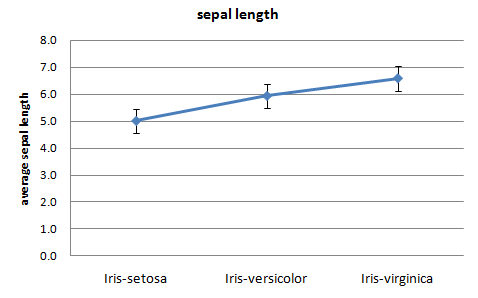
A line chart with error bars displays the mean of the numerical variable for each category of the categorical variable, connected by straight segments, with error bars showing the standard error of each mean. Overlapping bars signal that the group means may not be distinguishable; well-separated bars suggest a real difference. (Side-by-side box plots per category show the same comparison with full distribution detail.)

Combination Chart

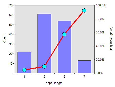
A combination chart pairs a bar chart of a binned numerical variable’s distribution with a line showing the percentage of a selected category of the categorical variable in each bin. It is the best visualization for demonstrating the predictive power of a numerical predictor (X-axis, binned) against a categorical target (Y-axis): a climbing or falling line means the variable separates the classes.

Z-Test and t-Test

The Z-test and t-test assess whether the averages of two groups are statistically different — appropriate for comparing a numerical variable across two categories. The Z-statistic measures the difference in means in units of standard error:

$Z = \frac{\bar{x}_1 - \bar{x}_2}{ \sqrt{ \frac{\sigma_1^2}{n_1} + \frac{\sigma_2^2}{n_2} } }$

A small probability for $Z$ means the difference between the averages is significant. When $n_1$ or $n_2$ is less than 30, use the t-test instead; with a pooled variance estimate,

$t = \frac{\bar{x}_1 - \bar{x}_2}{ s_p \sqrt{ \frac{1}{n_1} + \frac{1}{n_2} } }, \qquad s_p^2 = \frac{(n_1 - 1) s_1^2 + (n_2 - 1) s_2^2}{n_1 + n_2 - 2}$

compared against the t-distribution with $n_1 + n_2 - 2$ degrees of freedom.

Worked Example: O-Ring Failure and Temperature

Is there a significant difference in average temperature between launches with and without O-ring failure? The data:

O-Ring Failure	Temperature (°F)
Y	53, 56, 57, 70, 70, 70, 75
N	63, 66, 67, 67, 67, 68, 69, 70, 72, 73, 75, 76, 76, 78, 79, 80, 81

O-Ring Failure	Count	Mean	Variance
Y	7	64.43	76.95
N	17	72.18	30.78

With $n_1 = 7$ well under 30, the t-test applies:

$s_p^2 = \frac{6 \times 76.95 + 16 \times 30.78}{22} \approx 43.37, \qquad t = \frac{64.43 - 72.18}{\sqrt{43.37 \left( \frac{1}{7} + \frac{1}{17} \right)}} \approx -2.62$

with $df = 22$ and probability $p = 0.0156$. The low probability means the difference between the average temperature on failure days (64.43°F) and on intact days (72.18°F) is significant — failures happened on colder launches.

Analysis of Variance (ANOVA)

ANOVA assesses whether the averages of more than two groups differ statistically. It compares the variance between group means against the variance within groups:

$F = \frac{MS_B}{MS_W} = \frac{SS_B \, / \, (k - 1)}{SS_W \, / \, (N - k)}$

for $k$ groups and $N$ total observations. If group means were all equal, between-group variance would be small and $F \approx 1$; a large $F$ with a small probability indicates at least one group’s mean differs.

Worked Example: Humidity by Outlook

Is there a significant difference in average humidity across the three categories of Outlook in the golf dataset?

Outlook	Humidity values	Count	Mean	Variance
overcast	86, 65, 90, 75	4	79.0	127.3
rainy	96, 80, 70, 80, 91	5	83.4	104.8
sunny	85, 90, 95, 70, 70	5	82.0	132.5

Source of Variation	Sum of Squares	df	Mean Square	F	Probability
Between Groups	44.0	2	22.0	0.182	0.836
Within Groups	1331.2	11	121.0
Total	1375.2	13

The between-group mean square (22.0) is far smaller than the within-group mean square (121.0), so $F = 0.182$ with $p = 0.836$: there is no significant difference between the average humidity in the three Outlook categories. Knowing this upfront saves you from expecting Outlook to predict humidity in any later model.

In Practice

scipy.stats.ttest_ind and scipy.stats.f_oneway run these tests directly, and statsmodels provides full ANOVA tables via anova_lm. The combination chart’s logic — bin the predictor, plot the target rate per bin — is the same logic behind weight-of-evidence feature engineering in credit scoring and behind calibration plots for classifiers like sklearn.linear_model.LogisticRegression.

Common Pitfalls

• Using a Z-test on small samples — switch to the t-test below roughly 30 observations per group.
• Running many t-tests instead of one ANOVA — pairwise testing across $k$ groups inflates the false-positive rate.
• Ignoring variance heterogeneity — Welch’s t-test variant handles unequal variances better.
• Reading a significant $F$ as “all groups differ” — ANOVA only says at least one does; post-hoc tests localize it.
• Forgetting that significance is not size — with large $n$, tiny, useless differences reach $p \lt 0.05$.

Summary

A numerical variable against a categorical one is analyzed by comparing group distributions: error-bar and combination charts to see it, t-test (two groups) or ANOVA (three or more) to test it. The O-ring example shows a significant temperature difference ($t = -2.62$, $p = 0.0156$); the Outlook–humidity ANOVA shows a non-significant one ($F = 0.182$, $p = 0.836$) — both outcomes are equally informative before modeling.