Numerical vs. Numerical

Two numerical variables invite the most visual of all bivariate analyses: put one on each axis, draw one point per observation, and look. The scatter plot comes first; the correlation coefficient then compresses what you see into a single number.

Scatter Plot

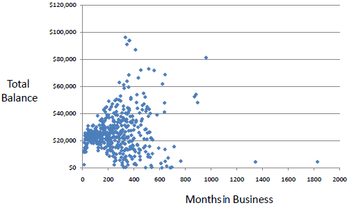
A scatter plot is a useful visual representation of the relationship between two numerical variables, and it is usually drawn before working out a linear correlation or fitting a regression line. The resulting pattern indicates the type (linear or non-linear) and the strength of the relationship: a tight diagonal cloud suggests strong linear association, a bent cloud a non-linear one, and a round blob no association at all.

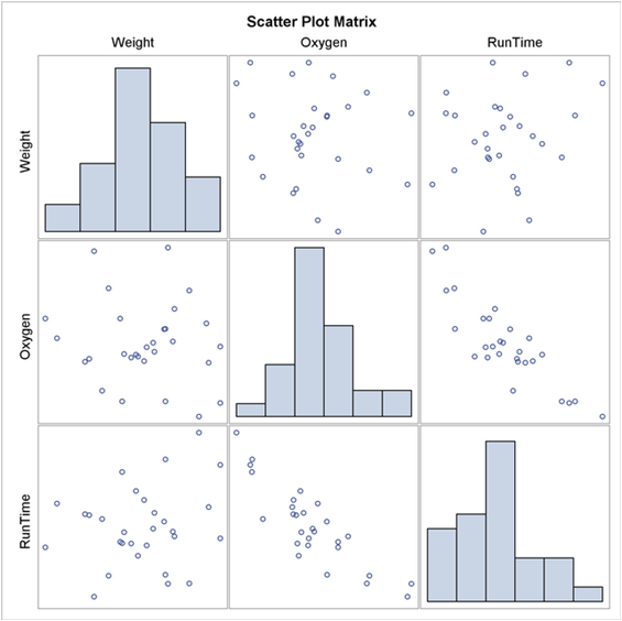
You can add information to a two-dimensional scatter plot — for example, labeling or coloring points to show the level of a third variable. With many variables in a dataset, the standard overview is a scatter plot matrix: all possible pairwise scatter plots arranged in a grid, so every numerical relationship gets one glance.

Linear Correlation

Linear correlation quantifies the strength of a linear relationship between two numerical variables. When there is no correlation, there is no tendency for the values of one quantity to increase or decrease with the values of the second. The Pearson correlation coefficient is the covariance of the two variables, normalized by their standard deviations:

$r = \frac{ \sum_{i=1}^{n} (x_i - \bar{x})(y_i - \bar{y}) }{ \sqrt{ \sum_{i=1}^{n} (x_i - \bar{x})^2 } \; \sqrt{ \sum_{i=1}^{n} (y_i - \bar{y})^2 } } = \frac{\mathrm{Cov}(x, y)}{s_x \, s_y}$

$r$ is always between −1 and 1: −1 means perfect negative linear correlation, +1 perfect positive, and 0 no linear correlation. It measures only linear strength — a perfect parabola scores near zero.

Worked Example: Temperature vs. Humidity

The legacy example uses the 14 days of the Play Golf dataset, this time with the raw numerical values of temperature and humidity:

Day	1	2	3	4	5	6	7	8	9	10	11	12	13	14
Temperature	83	64	72	81	70	68	65	75	71	85	80	72	69	75
Humidity	86	65	90	75	96	80	70	80	91	85	90	95	70	70

The means are $\bar{x} = 73.57$ (temperature) and $\bar{y} = 81.64$ (humidity). Computing the moments around those means (dividing by $n$):

	Variance	Covariance	Correlation
Temperature	40.10	19.78	0.32
Humidity	98.23

The positive covariance says the variables move in the same direction on average; normalizing gives

$r = \frac{19.78}{\sqrt{40.10} \cdot \sqrt{98.23}} \approx 0.32,$

a weak positive linear correlation between temperature and humidity. Hotter days tended to be slightly more humid in this sample, but the relationship explains little of the variation — consistent with the loose cloud in the scatter plot.

In Practice

df.corr() produces the full correlation matrix in pandas, scipy.stats.pearsonr adds a p-value, and sns.pairplot renders the scatter plot matrix. Correlation analysis is a standard feature-screening step: drop one of two near-perfectly correlated predictors (multicollinearity hurts linear models), but remember that tree ensembles like XGBoost are insensitive to monotone transformations and can exploit non-linear structure that $r$ misses entirely.

Common Pitfalls

• Equating $r = 0$ with independence — non-linear relationships are invisible to Pearson’s $r$.
• Ignoring outliers. A single extreme point can manufacture or destroy a correlation; check the plot.
• Confusing correlation with causation, especially in time-linked data with trends.
• Comparing $r$ across different ranges — restricting the range of $x$ mechanically shrinks $r$.
• Reporting $r$ without $n$. A correlation of 0.9 on 5 points means far less than 0.4 on 5,000.

Summary

Scatter plots reveal the form and strength of a two-numerical-variable relationship; the Pearson coefficient compresses the linear part into a number between −1 and 1. The temperature–humidity example shows the workflow end to end: plot, compute covariance, normalize, and interpret — here landing on a weak $r \approx 0.32$.