Categorical vs. Categorical

When both variables are categorical, bivariate analysis is built on one object: the contingency table (cross-tabulation), which counts observations for every combination of categories. From it flow the visualizations — stacked column and combination charts — and the chi-square test, the classical answer to “are these two variables associated?”

Stacked Column Chart

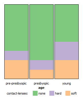
A stacked column chart compares the percentage that each category of one variable contributes to a total across the categories of the second variable. Each column is one category of the predictor, split into segments by the target’s categories — differences in segment heights between columns are the visual signature of an association.

Combination Chart

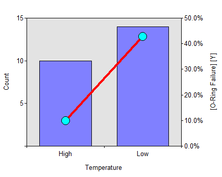
A combination chart uses two chart types to show different kinds of information at once. Here, bars show the distribution of one categorical variable while a line shows the percentage of a selected category of the second variable. It is the best visualization for demonstrating the predictive power of a predictor (X-axis) against a target (Y-axis): if the line is flat, the predictor tells you nothing; the more it tilts, the more the categories separate the target.

Chi-Square Test

The chi-square test determines whether two categorical variables are associated. It is based on the difference between the observed frequencies $n_{ij}$ and the frequencies $e_{ij}$ you would expect if the variables were independent. Under independence, the expected count for cell $(i, j)$ is the row total times the column total, divided by the grand total:

$e_{ij} = \frac{n_{i\cdot} \cdot n_{\cdot j}}{n}$

The test statistic accumulates the squared discrepancy over every cell of the contingency table:

$\chi^2 = \sum_{i,j} \frac{(n_{ij} - e_{ij})^2}{e_{ij}}$

with degrees of freedom $df = (r - 1)(c - 1)$ for a table with $r$ rows and $c$ columns. The chi-square distribution converts the statistic to a probability $p$: a probability near zero indicates dependency between the variables, while a probability near one means they are essentially independent.

To measure the strength of the dependency (the chi-square statistic grows with sample size, so it is not itself a strength measure), the legacy page uses the Tchouproff contingency coefficient:

$\rho_\tau = \sqrt{ \frac{\chi^2}{n \sqrt{(r - 1)(c - 1)}} }$

Worked Example: Hair Color vs. Eye Color

The legacy example cross-tabulates hair color against eye color for 95 people. Expected frequencies under independence appear in parentheses:

Eye color	Light hair	Dark hair	Row total
Black	32 (24.1)	12 (19.9)	44
Green/Blue	14 (19.7)	22 (16.3)	36
Others	6 (8.2)	9 (6.8)	15
Column total	52	43	95

Walk one cell: the expected count for black eyes and light hair is $\frac{44 \times 52}{95} = 24.1$, contributing $\frac{(32 - 24.1)^2}{24.1} \approx 2.6$ to the statistic. Summing all six cells:

$\chi^2 \approx 10.67, \qquad df = (3 - 1)(2 - 1) = 2, \qquad p = 0.005$

The low probability (0.005) shows a significant dependency between hair color and eye color. The Tchouproff coefficient,

$\rho_\tau = \sqrt{\frac{10.67}{95 \sqrt{2 \cdot 1}}} \approx 0.28,$

indicates a moderate-strength association — real, but far from deterministic.

In Practice

pd.crosstab(df.a, df.b) builds the table and scipy.stats.chi2_contingency returns the statistic, p-value, degrees of freedom, and expected frequencies in one call. In machine learning, the same idea powers sklearn.feature_selection.chi2, which ranks categorical predictors against a categorical target, and information-gain measures in decision trees are close cousins of the dependency measured here.

Common Pitfalls

• Applying chi-square to tiny expected counts — the approximation breaks down silently.
• Reading the p-value as strength. With large $n$, trivial associations reach $p \lt 0.001$; report an effect size like $\rho_\tau$ or Cramér’s V alongside.
• Chi-square on raw numerical data — bin first (see Binning), and know that binning choices affect the result.
• Ignoring the table for the test. The cells with the largest $(n - e)$ gaps tell you where the association lives; read them.
• Claiming causation from an association in observational data.

Summary

Two categorical variables are analyzed through the contingency table: stacked and combination charts make the association visible, and the chi-square test measures its significance against the independence hypothesis, with coefficients like Tchouproff’s quantifying strength. The hair/eye example shows the full workflow — table, expected counts, $\chi^2 = 10.67$ on 2 degrees of freedom, $p = 0.005$ — from raw counts to a defensible conclusion.