Linear Discriminant Analysis

Linear Discriminant Analysis (LDA), introduced by R. A. Fisher in 1936, searches for a linear combination of the predictors that best separates two classes. It is simple, mathematically robust, and — when the classes are roughly Gaussian with shared covariance — often as accurate as far more complex methods.

Unlike logistic regression, which models the posterior probability directly, LDA models each class distribution and derives the separating boundary from their geometry.

Fisher’s criterion

The idea: project the data onto a direction $w$ so that the projected class means are far apart while the projected within-class scatter is small. Fisher captured this as a score to maximize — the ratio of between-class scatter to within-class scatter:

$J(w) = \frac{w^{T} S_B\, w}{w^{T} S_W\, w}$

For two classes with means $\mu_1$ and $\mu_2$:

$S_B = (\mu_1 - \mu_2)(\mu_1 - \mu_2)^{T}$

$S_W = \sum_{x_i \in C_1} (x_i - \mu_1)(x_i - \mu_1)^{T} + \sum_{x_i \in C_2} (x_i - \mu_2)(x_i - \mu_2)^{T}$

Maximizing $J(w)$ has a closed-form solution — no iterative fitting required:

$w \;\propto\; S_W^{-1}\, (\mu_1 - \mu_2)$

A new point $x$ is classified by projecting it onto this maximally separating direction and comparing the score $z = w^T x$ against a threshold $z_0$ derived from the projected class means and priors: assign $C_1$ if $z > z_0$, otherwise $C_2$.

Worked example: small-business default

A bank provides data on small-business clients who defaulted and those who did not, described by two predictors: delinquent days (DAYSDELQ) and months in business (BUSAGE). LDA fits the optimal linear model separating default (Y) from non-default (N).

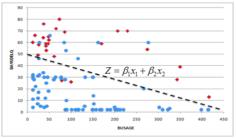
The computation proceeds in three steps:

1. Class statistics. Compute the mean vector and covariance matrix of each class, plus the class priors.
2. Pooled covariance. Average the class covariances into a single pooled matrix $\Sigma$ and invert it.
3. Coefficients. The discriminant direction is $w = \Sigma^{-1}(\mu_1 - \mu_2)$, giving a linear score $z$ in the two predictors.

For this dataset the Mahalanobis distance between the classes is 2.32 — modest but usable separation. Scoring each client and classifying N when the score exceeds the threshold of −1.1, the model misclassifies just 2 of the training cases.

Which predictors matter?

Correlate each predictor with the model’s discriminant scores. A correlation near −1 or 1 means the predictor drives the separation (the sign only sets direction); a correlation near 0 means it contributes nothing to the discriminant function.

Quadratic Discriminant Analysis

QDA relaxes LDA’s shared-covariance assumption, estimating a separate covariance matrix $\Sigma_k$ per class. The discriminant function becomes quadratic in $x$:

$\delta_k(x) = -\tfrac{1}{2} \ln |\Sigma_k| - \tfrac{1}{2}(x - \mu_k)^{T} \Sigma_k^{-1} (x - \mu_k) + \ln P(c_k)$

and the classification rule is simply $\arg\max_k \delta_k(x)$. QDA is more flexible — curved decision boundaries — but estimates many more parameters, so it needs more data per class to stay stable.

In practice

sklearn.discriminant_analysis.LinearDiscriminantAnalysis and QuadraticDiscriminantAnalysis cover both variants; LDA also doubles as a supervised dimensionality-reduction method via its transform. LDA remains a strong baseline when classes are well separated and roughly Gaussian, and it is a standard preprocessing step before feeding compact discriminants into other models. For high-dimensional data, use the shrinkage solver (solver='lsqr', shrinkage='auto') to regularize the covariance estimate.

Common pitfalls

• Non-Gaussian or heavily skewed classes. LDA’s optimality rests on Gaussian classes with equal covariance; strong violations degrade it.
• Unequal covariances. If class spreads differ markedly, switch to QDA rather than forcing a linear boundary.
• Singular covariance. With more predictors than observations — or collinear predictors — $S_W$ can’t be inverted without regularization.
• Reading coefficients like correlations. Standardize predictors first if you want comparable coefficient magnitudes.

Summary

LDA finds the projection direction that maximizes the ratio of between-class to within-class scatter, with the closed-form solution $w \propto S_W^{-1}(\mu_1 - \mu_2)$. Classification is projection plus threshold, and the Mahalanobis distance tells you how separable the classes really are. When classes have different shapes, QDA trades a linear boundary for a quadratic one at the cost of estimating more parameters.