Decision Tree

A decision tree breaks a dataset into smaller and smaller subsets while incrementally growing an associated tree of decisions. The result is a structure of decision nodes, each testing one attribute, and leaf nodes, each holding a final classification. The topmost decision node — the best single predictor — is the root node.

Trees handle both categorical and numerical data, are easy to read, and double as a set of human-checkable rules. Where Naive Bayes assumes predictors are independent, a decision tree explicitly models their interactions: each split is asked in the context of the splits above it.

The ID3 algorithm

The core tree-building algorithm is ID3 (J. R. Quinlan): a top-down, greedy search that picks the best split at each node and never backtracks. “Best” is measured with entropy and information gain.

For a set $S$ with classes $1 \dots c$ and class proportions $p_i$:

$E(S) = \sum_{i=1}^{c} -p_i \log_2 p_i$

Information gain is the decrease in entropy after splitting $S$ on an attribute $A$:

$IG(S, A) = E(S) - \sum_{v \in \text{Values}(A)} \frac{|S_v|}{|S|}\, E(S_v)$

where $S_v$ is the subset of $S$ for which attribute $A$ has value $v$. ID3 chooses the attribute with the highest information gain, splits, and recurses on every branch until each branch is pure (entropy 0).

Worked example: Play Golf

Using the same 14-row dataset as Naive Bayes — 9 Yes and 5 No overall:

Step 1 — entropy of the target.

$E(S) = -\frac{9}{14}\log_2\frac{9}{14} - \frac{5}{14}\log_2\frac{5}{14} = 0.940$

Step 2 — entropy and gain for every attribute.

Attribute	Branch entropies	Weighted entropy	Information gain
Outlook	Sunny 0.971 (5 rows) · Overcast 0 (4) · Rainy 0.971 (5)	0.693	0.247
Humidity	High 0.985 (7) · Normal 0.592 (7)	0.789	0.152
Windy	False 0.811 (8) · True 1.000 (6)	0.892	0.048
Temp	Hot 1.000 (4) · Mild 0.918 (6) · Cool 0.811 (4)	0.911	0.029

For example, Outlook’s weighted entropy is $\frac{5}{14}(0.971) + \frac{4}{14}(0) + \frac{5}{14}(0.971) = 0.693$, so $IG(S, \text{Outlook}) = 0.940 - 0.693 = 0.247$.

Step 3 — pick the largest gain. Outlook wins, so it becomes the root node. Divide the dataset into its three branches and repeat on each.

Step 4 — leaf or recurse. The Overcast branch is all Yes: entropy 0, a leaf. The Sunny branch (3 Yes, 2 No, $E = 0.971$) and the Rainy branch (2 Yes, 3 No, $E = 0.971$) need further splitting.

Step 5 — recurse.

• Sunny subset: gains are Windy 0.971, Humidity 0.020, Temp 0.020. Windy separates perfectly — Windy = False is all Yes (3 rows), Windy = True is all No (2 rows).
• Rainy subset: gains are Humidity 0.971, Temp 0.571, Windy 0.020. Humidity separates perfectly — High is all No (3 rows), Normal is all Yes (2 rows).

Every branch is now pure, and the algorithm stops.

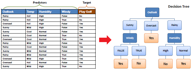
Transcribed as rules, the tree is:

• Outlook = Overcast → Play Golf = Yes (4/4)
• Outlook = Sunny
  • Windy = False → Yes (3/3)
  • Windy = True → No (2/2)
• Outlook = Rainy
  • Humidity = High → No (3/3)
  • Humidity = Normal → Yes (2/2)

Interactive builder: step through ID3 on this dataset — entropy of each subset, information gain of each candidate split, and the tree growing one node at a time. The final tree it converges to:

• Outlook?
  • Overcast → Yes (4/4)
  • Sunny → Windy?
    • False → Yes (3/3)
    • True → No (2/2)
  • Rainy → Humidity?
    • High → No (3/3)
    • Normal → Yes (2/2)

From tree to rules

Any decision tree converts directly into a set of if–then rules by tracing each root-to-leaf path, e.g. IF Outlook = Sunny AND Windy = False THEN Play Golf = Yes. Rules are often easier to audit and hand to domain experts than the tree diagram itself.

In practice

Modern libraries implement ID3’s descendants: C4.5 (gain ratio, pruning, continuous splits) and CART (Gini impurity, binary splits) — sklearn.tree.DecisionTreeClassifier is CART. Single trees are rarely the final model today; they shine as the base learners of ensembles. Random forests average many decorrelated trees, and gradient-boosted trees (XGBoost, LightGBM) add them sequentially to correct prior errors — routinely the strongest off-the-shelf models on tabular data. Explain a fitted tree with sklearn.tree.export_text, or an ensemble with SHAP values.

Common pitfalls

• Overfitting. An unpruned tree memorizes noise. Limit depth, require minimum samples per leaf, or prune.
• Super attributes. An attribute with many unique values (an ID column) has huge information gain but zero predictive power — the reason C4.5 introduced gain ratio.
• Instability. Tiny data changes can flip the root split and restructure the whole tree. Ensembles fix this; a single tree does not.
• Continuous attributes. ID3 needs them discretized; C4.5/CART find optimal thresholds automatically.
• Ignoring class imbalance. With skewed classes, accuracy-maximizing splits can ignore the minority class entirely.

Summary

ID3 builds a decision tree greedily: compute the entropy of the target, pick the attribute with the highest information gain, split, and recurse until every branch is pure. The Play Golf dataset splits on Outlook at the root (gain 0.247), then Windy under Sunny and Humidity under Rainy. The result is a compact, rule-equivalent model — and the foundation of the ensemble methods that dominate tabular prediction.