Evaluation: Classification

A classification model’s performance is summarized by counting how its predictions line up against the actual outcomes. Every metric on this page — accuracy, precision, recall, specificity, F1, ROC, AUC — is arithmetic over four counts. Learn the four counts and the rest follows. These metrics assume an honest train/test protocol; see Model Evaluation for that.

The confusion matrix

A confusion matrix shows the number of correct and incorrect predictions made by the model compared to the actual outcomes in the data. For two classes (Positive and Negative) it is a $2 \times 2$ table:

	Target: Positive	Target: Negative
Model: Positive	$a$ (true positive)	$b$ (false positive)
Model: Negative	$c$ (false negative)	$d$ (true negative)

Five standard metrics read directly off the cells:

$$\text{Accuracy} = \frac{a + d}{a + b + c + d} \qquad \text{Precision (PPV)} = \frac{a}{a + b} \qquad \text{NPV} = \frac{d}{c + d}$$ $$\text{Sensitivity (Recall)} = \frac{a}{a + c} \qquad \text{Specificity} = \frac{d}{b + d}$$

• Accuracy — the proportion of all predictions that were correct.
• Precision (positive predictive value) — of the cases the model called positive, the proportion that truly were.
• Negative predictive value — of the cases the model called negative, the proportion that truly were.
• Sensitivity (recall, true positive rate) — of the actual positive cases, the proportion the model caught.
• Specificity (true negative rate) — of the actual negative cases, the proportion the model correctly left alone.

Precision and sensitivity pull in opposite directions: flagging everything as positive gives perfect sensitivity and terrible precision. The F1 score is their harmonic mean, a single number that stays low unless both are high:

$$F_1 = \frac{2 \cdot \text{Precision} \cdot \text{Sensitivity}}{\text{Precision} + \text{Sensitivity}}$$

Worked example

A model is evaluated on 200 cases: 100 truly positive, 100 truly negative.

| | Target: Positive | Target: Negative | | | --- | --- | --- | --- | --- | | Model: Positive | $a = 70$ | $b = 20$ | PPV $= 70/90 \approx 0.78$ | | Model: Negative | $c = 30$ | $d = 80$ | NPV $= 80/110 \approx 0.73$ | | | Sensitivity $= 70/100 = 0.70$ | Specificity $= 80/100 = 0.80$ | Accuracy $= 150/200 = 0.75$ |

Reading row-wise and column-wise gives every metric. PPV looks along the predicted-positive row: $70/(70+20) \approx 0.78$. Sensitivity looks down the truly-positive column: $70/(70+30) = 0.70$. The F1 score combines the two:

$$F_1 = \frac{2 \cdot 0.78 \cdot 0.70}{0.78 + 0.70} \approx 0.74$$

Gain, lift, and K-S charts

A confusion matrix evaluates the model over the whole population at one threshold. When only a fraction of the population will be acted on — say, the 10% of customers most likely to respond — three older diagnostic charts help:

• Gain chart: sort cases by model score and plot the cumulative percentage of positives captured against the percentage of population contacted.
• Lift chart: the ratio of positives captured with the model versus random selection at each depth; a lift of 3 at 10% depth means contacting the top decile reaches three times as many respondents as a random 10%.
• K-S (Kolmogorov–Smirnov) chart: the maximum separation between the cumulative positive and negative score distributions; 0 means no separation, 100 means perfect separation.

ROC curve and AUC

Most classifiers output a score, not a hard class; the confusion matrix appears only after you pick a threshold. The ROC chart sidesteps the choice: it plots the true positive rate (sensitivity) against the false positive rate ($1 - \text{specificity}$) at every threshold. A good model’s curve climbs quickly toward the top-left corner; the diagonal is a random model.

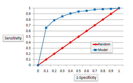
The area under the ROC curve (AUC) compresses the curve into one number. A random classifier has AUC $= 0.5$; a perfect one has AUC $= 1$. The interpretation is probabilistic: an AUC of 0.8 means a randomly chosen positive case outranks a randomly chosen negative case 80% of the time.

Try the interaction between threshold, confusion matrix, and ROC curve directly:

With the worked example above scored at threshold 0.5, the confusion matrix is TP = 70, FP = 20, FN = 30, TN = 80, giving:

• True positive rate (sensitivity): 70 / (70 + 30) = 0.70
• False positive rate: 20 / (20 + 80) = 0.20
• Accuracy: 0.75, precision: 0.78, F1: 0.74

Raising the threshold shrinks both rates (fewer positive calls); lowering it grows both. The ROC curve is the trace of the (FPR, TPR) operating point across all thresholds; AUC summarizes it — 0.5 is random, 1.0 is perfect.

In practice

Modern metric practice goes beyond reporting accuracy at the default 0.5 threshold. Choose the threshold from the costs of the two error types — a cancer screen accepts more false positives than a spam filter — and tune it on validation data, never the test set. Under class imbalance, accuracy is actively misleading: a fraud model that never fires scores 99.9% accuracy on 0.1% fraud, so report precision, recall, and F1 on the minority class instead. When positives are rare, prefer the precision–recall curve and its area (average_precision_score) over ROC — ROC’s false-positive-rate axis can look reassuringly small even when most positive calls are wrong. In scikit-learn, sklearn.metrics.classification_report prints per-class precision/recall/F1, roc_auc_score and RocCurveDisplay handle ROC/AUC, and precision_recall_curve plus confusion_matrix cover threshold analysis; SHAP or permutation importance then explain what the model got right.

Common pitfalls

• Reporting accuracy on imbalanced data — always pair it with per-class precision and recall.
• Tuning the threshold on the test set — the resulting metrics are no longer honest estimates; use a validation split or cross-validation.
• Comparing models at different thresholds — fix the operating point or compare full ROC/PR curves.
• Assuming 0.5 is the right cutoff — for most score distributions it is arbitrary.
• Reading precision off a different population — PPV and NPV shift with the base rate of positives; sensitivity and specificity do not.

Summary

The confusion matrix reduces a classifier to four counts, from which accuracy, precision, NPV, sensitivity, specificity, and F1 are simple fractions. Gain, lift, and K-S charts evaluate ranked subsets of the population, while the ROC curve and AUC summarize performance across every threshold. In modern practice the threshold is a deliberate business decision, and precision–recall analysis replaces ROC when positives are rare.