Logistic Regression

Logistic regression predicts the probability of an outcome that can take only two values — default or not, churn or not, disease or not — from any mix of numerical and categorical predictors. Despite the name, it is a classification model, and it remains the default baseline for binary outcomes because its coefficients are directly interpretable.

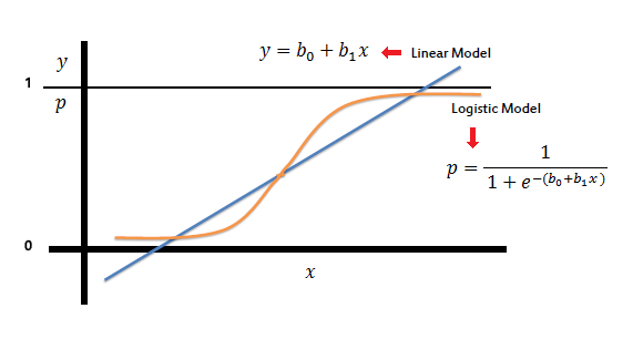
Ordinary linear regression is the wrong tool here for two reasons: it can predict probabilities outside $[0, 1]$, and with a binary target the residuals are never normally distributed around the fitted line. Logistic regression fixes both by fitting a sigmoid instead of a line.

The sigmoid and the logit

The logistic curve squashes any real-valued score into the range 0 to 1:

$p(x) = \frac{1}{1 + e^{-(b_0 + b_1 x)}}$

The constant $b_0$ shifts the curve left and right; the slope $b_1$ controls its steepness.

Dividing through by $1 - p$ gives a simple statement about the odds:

$\frac{p}{1 - p} = e^{\,b_0 + b_1 x}$

and taking the natural logarithm makes the relationship linear in the predictors. This is the logit (log-odds):

$\ln \frac{p}{1 - p} = b_0 + b_1 x$

The coefficient $b_1$ is the change in log-odds per one-unit increase in $x$; exponentiated, $e^{b_1}$ is the odds ratio — the factor by which the odds multiply per unit of $x$. The model extends to any number of predictors:

$\ln \frac{p}{1 - p} = b_0 + b_1 x_1 + b_2 x_2 + \dots + b_k x_k$

The decision boundary sits where $p = 0.5$, i.e. where the logit equals 0 — a linear surface in the predictors, just like LDA.

Fitting: maximum likelihood

Where linear regression minimizes squared error, logistic regression chooses coefficients by maximum likelihood estimation (MLE): find the $b$ values that maximize the probability of observing the actual outcomes. The log-likelihood is

$LL = \sum_{i=1}^{n} \Big[ y_i \ln p_i + (1 - y_i) \ln (1 - p_i) \Big]$

and it is maximized iteratively (the optimizer repeats until $LL$ stops improving). Three diagnostics then assess the fit:

• Pseudo $R^2$. Several measures mimic $R^2$ for logistic models, but they disagree with each other and can’t be read like $R^2$:

  Measure	Idea
  Efron’s	Squared residuals summed and divided by total variability in the target
  McFadden’s	$1 - \dfrac{LL_{\text{full}}}{LL_{\text{intercept}}}$ — improvement of the full model over an intercept-only model
  Count	Fraction of records correctly predicted at a 0.5 cutoff — plain accuracy

• Likelihood ratio test. Compares the full model against a restricted (e.g. intercept-only) model: $G = -2\,(LL_{\text{reduced}} - LL_{\text{full}})$ follows a $\chi^2$ distribution with degrees of freedom equal to the difference in parameter counts. It answers “does the model as a whole beat the baseline?”

• Wald test. Tests each coefficient individually: $W = \dfrac{b}{SE}$ is approximately normal, and $W^2$ is $\chi^2$ with one degree of freedom. It answers “does this predictor contribute?”

Worked example: interpreting coefficients

Fitting the bank default data (predictors DAYSDELQ and BUSAGE, target DEFAULT) yields coefficients of roughly $b_1 = 0.102$ for DAYSDELQ and $b_2 = 0.008$ for BUSAGE. Interpretation via odds ratios:

• One more delinquent day multiplies the odds of default by $e^{0.102} \approx 1.11$ — about an 11% increase in the odds, all else fixed.
• One more month in business multiplies the odds by $e^{0.008} \approx 1.008$ — about a 0.8% increase.

Signs, magnitudes, and odds ratios make logistic models uniquely easy to explain to non-technical stakeholders — a major reason the method endures.

In practice

sklearn.linear_model.LogisticRegression is the standard implementation; use LogisticRegressionCV to tune the regularization strength $C$ by cross-validation. Standardize numeric predictors (StandardScaler in a Pipeline) so coefficients are comparable and regularization treats them fairly. The model’s predicted probabilities are usually well calibrated out of the box, which makes it the reference point when evaluating probability-producing classifiers like naive Bayes. For high-dimensional sparse data (text), L1-penalized logistic regression doubles as a feature selector.

Common pitfalls

• Reading $e^b$ as a probability change. It is an odds multiplier, not a percentage-point shift in probability — the effect on $p$ depends on the baseline.
• Perfect separation. If a predictor (or combination) separates the classes completely, MLE diverges and coefficients blow up; use penalization.
• Multicollinearity. Correlated predictors inflate standard errors and make Wald tests unreliable.
• Comparing pseudo $R^2$ variants. McFadden’s, Efron’s, and Count $R^2$ measure different things and can rank models differently — pick one and state which.
• Forcing a 0.5 cutoff. The threshold is a business decision; choose it with the confusion matrix and ROC analysis, not by default.

Summary

Logistic regression models the log-odds of a binary outcome as a linear function of the predictors, then maps that score back to a probability through the sigmoid. Coefficients are fit by maximum likelihood and read as odds ratios; overall fit is judged by likelihood-ratio tests and pseudo $R^2$, individual predictors by the Wald test. It is interpretable, well calibrated, and still the baseline every fancier classifier must beat.